GPR Utility Locating: Depth & Soil Limits
How GPR finds metallic and nonmetallic lines from dielectric contrast, how antenna frequency trades depth for resolution, and where wet clay limits a scan.
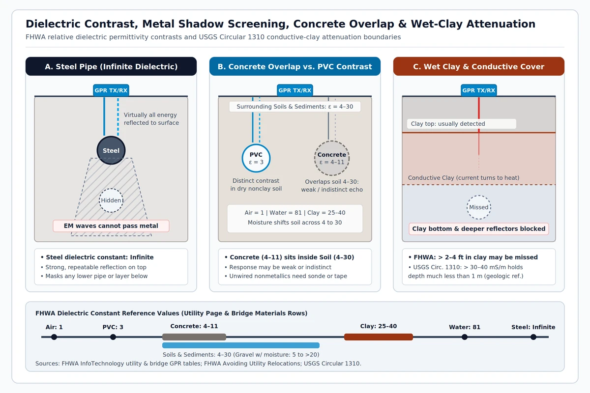
Ground-penetrating radar (GPR) sends high-frequency electromagnetic pulses into the ground and maps subsurface anomalies from shifts in electrical conductivity and relative dielectric permittivity. Because electromagnetic waves cannot penetrate metals such as steel or cast-iron pipe, a metal utility reflects virtually all incident energy and creates a shadow zone that hides any feature directly beneath it. Nonmetallic utilities register clearly in dry, nonclay ground when their permittivity contrasts sharply with surrounding soil, whereas concrete storm and sewer pipes sit inside the typical soil permittivity span and often return weak or indistinct echoes. Wet or clay-rich soils rapidly attenuate radar energy—once clay content rises, utilities deeper than 2 to 4 feet routinely go undetected.
In pre-excavation site work, gpr utility locating works alongside electromagnetic line tracing and physical potholing rather than replacing either step. Coordinate underground utility sweeps with the broader smart jobsite and survey technology workflow across our civil and jobsite engineering reference. Resolving duct, pipe, and structural clearances inside coordinated 3D models belongs to the BIM clash detection and MEP coordination guide, while GNSS base-station setup and blade verification during earthwork belong to the machine control grading checks guide.
How does GPR detect metallic and nonmetallic underground lines?
Two electrical properties control every radar pass: electrical conductivity (the inverse of resistivity) governs how far electromagnetic energy penetrates into the ground, while relative dielectric permittivity (dielectric constant) controls wave propagation speed (FHWA InfoTechnology underground utility GPR reference). Wherever adjacent materials differ in dielectric constant, the resulting impedance boundary reflects part of the pulse back to the receiving antenna—allowing a B-scan record to pick up metal mains, nonmetallic conduits, air voids, and disturbed trench backfill (FHWA Avoiding Utility Relocations, Section IV).
Every subsurface material is electromagnetically defined by permittivity, magnetic permeability, and electrical conductivity, so radar detection requires a measurable contrast in at least one of those three parameters between the buried target and surrounding host soil (NIST buried-object detection report). When ground propagation velocity is calibrated or estimated, two-way wave arrival times convert directly into interface depth (ASTM D6432-19).
Physical end members set the upper and lower contrast boundaries on a utility scan. A vacuum has a relative dielectric constant of 1 (air is essentially the same at 1), the lowest possible value, whereas metals such as steel act as effectively perfect conductors with infinite effective permittivity and reflect virtually all incoming electromagnetic energy. That upper boundary makes steel pipe responses strong and repeatable while blocking radar waves from imaging any deeper line stacked directly underneath. Concrete pipes present the opposite challenge: at a relative dielectric constant of 4 to 11, concrete sits squarely inside the 4 to 30 range of ordinary soils and sediments, so concrete pipe crowns often blend into surrounding backfill unless an air space inside the pipe boosts contrast.
| Material | Relative dielectric constant | Subsurface reflection and contrast behavior |
|---|---|---|
| Air | 1 | Lowest permittivity boundary; air voids inside dry conduits or culverts produce sharp reflections against damp backfill. |
| PVC | 3 | Distinct permittivity contrast in dry, nonclay sand or silt when surrounding ground moisture stays moderate. |
| Concrete | 4 to 11 | Overlaps soils and sediments (4 to 30), so concrete storm and sewer pipe echoes can be weak or indistinguishable from native ground. |
| Soils and sediments | 4 to 30 | Pore moisture shifts bulk soil permittivity across a wide 4 to 30 span and alters depth-conversion velocity. |
| Clay | 25 to 40 | High permittivity paired with high electrical conductivity; moist gravel on the FHWA bridge-deck GPR materials table similarly shifts from 5 to above 20. |
| Water | 81 | Sharpest nonmetallic reflector; localized shifts in soil water content generate many of the strongest subsurface GPR reflections. |
| Steel | Infinite | Acts as a perfect conductor, reflecting incident radar energy and masking deeper utilities directly below the pipe. |
How deep can ground-penetrating radar scan for buried utilities?
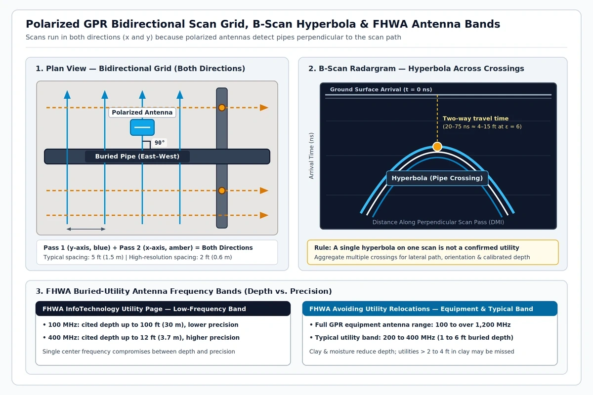
Antenna center frequency sets the fundamental tradeoff between scan depth and target resolution. Lower center frequencies penetrate deeper with coarser spatial resolution, whereas higher center frequencies resolve smaller conduits at shallower depths—forcing crews running a single-frequency cart to balance reach against clarity.
Across geophysical applications, surface GPR instruments span 10 to 7,000 MHz (ASTM D6432-19), with utility carts operating in a much narrower band tailored to typical trench depths:
- 100 to 400 MHz low-frequency utility range: Cited on the FHWA InfoTechnology utility GPR page with upper-bound penetration up to 100 ft (30 m) at 100 MHz under ideal low-loss ground and up to 12 ft (3.7 m) at 400 MHz.
- 200 to 400 MHz standard utility cart band: Within a broader 100 to over 1,200 MHz equipment family, 200 to 400 MHz antennas are the workhorse choice for resolving buried utilities across the typical 1 to 6 ft (0.3 to 1.8 m) burial zone (FHWA Avoiding Utility Relocations, Section IV).
Nominal antenna ratings never guarantee depth on an active jobsite. Actual detection depends on burial depth, pipe diameter, pipe deterioration, trench backfill contrast, surface pavement, and—above all—soil conductivity. Wet clay and saline or saturated subgrades convert induced electromagnetic currents into heat, collapsing effective scan depth. Once clay content climbs, 200 to 400 MHz utility scans routinely miss lines deeper than 2 to 4 feet.
Field conductivity thresholds explain why clay caps shut down radar surveys so abruptly. Effective GPR penetration generally requires ground electrical conductivity below 40 mS/m (resistivity above 25 ohm-meters), as radar amplitude decays through spherical spreading, conductive heat loss, and coarse-clast scattering (USGS Circular 1310). While low-conductivity dry sand and gravel can pass low-frequency signals to 15–20 m at 0.5–1.5 m geologic resolution, radar waves usually detect only the top boundary of a clay horizon while failing to image the clay base or any reflector beneath it. Where surface soil conductivity exceeds 30 to 40 mS/m, penetration often drops well below 1 m unless the conductive clay cap is stripped first.
What equipment and grid setup are used for GPR utility mapping?
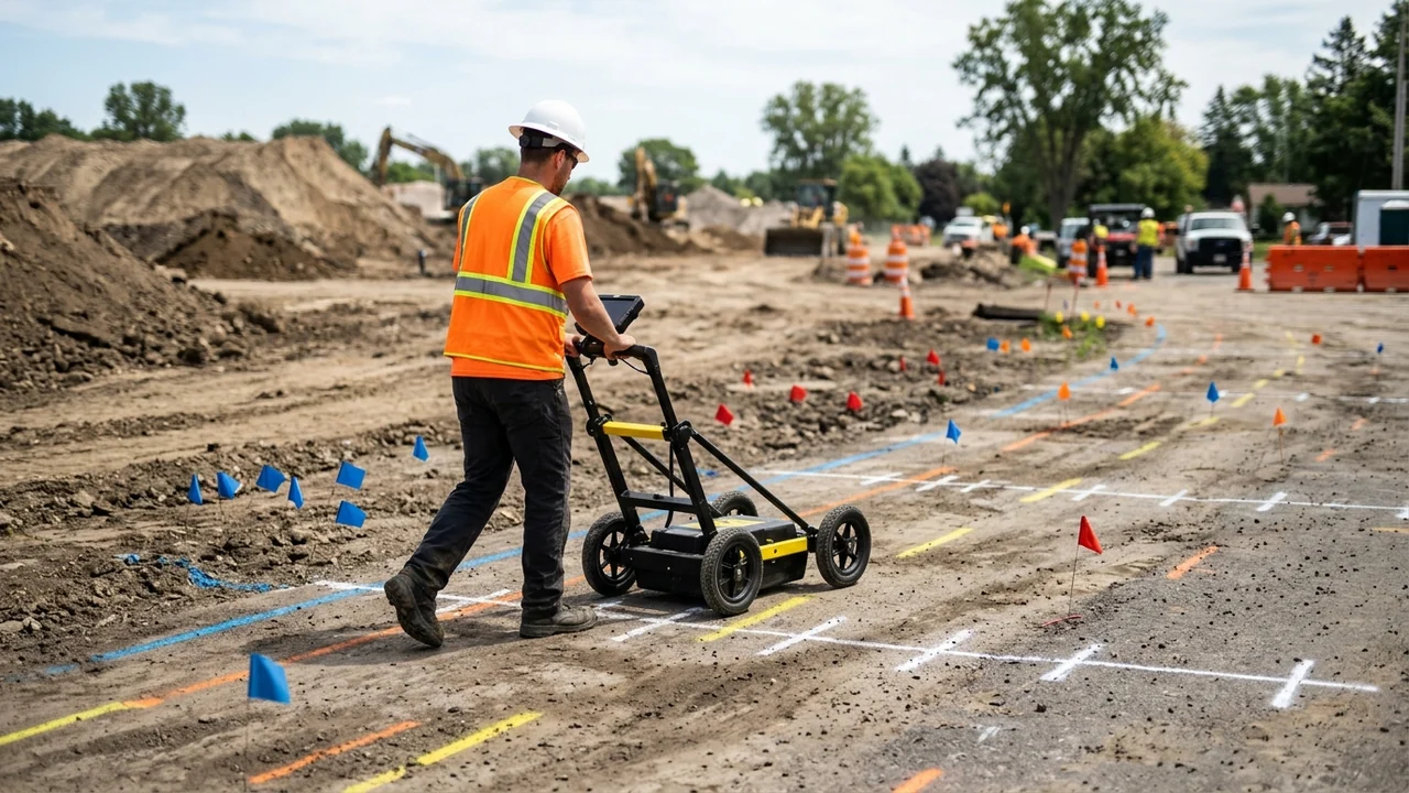
A standard ground penetrating radar construction cart pairs a shielded radar antenna with a digital data acquisition unit, a wheel-mounted distance measurement instrument (DMI) that paces trace intervals, and a GNSS/GPS receiver (FHWA InfoTechnology utility GPR reference). Utility crews pull ground-coupled antennas flush against pavement or graded soil for maximum energy transfer, whereas air-coupled horn antennas ride 1 to 2 ft (0.3 to 0.6 m) above the surface for high-speed corridor passes. Pairing GNSS with the DMI georeferences the horizontal cart track for CAD and GIS overlays, though surface coordinates never turn an unverified radar reflection into a survey-grade pipe invert.
Reliable utility detection depends on grid geometry and disciplined B-scan interpretation:
- Collect a bidirectional x- and y-grid: Because standard GPR dipoles are polarized and respond strongest when crossing a linear target at 90 degrees, runs must cover both perpendicular axes so longitudinal and transverse mains register equally.
- Match traverse spacing to target complexity: Standard utility grids use 5 ft (1.5 m) line spacing in both directions, tightened to 2 ft (0.6 m) across congested intersections or critical tie-ins. Broad reconnaissance sweeps for undocumented lines combine electromagnetic induction, passive scanning, and GPR along street-parallel and street-perpendicular passes every 5 to 20 feet (FHWA Avoiding Utility Relocations, Section IV).
- Set realistic time windows and calibrate soil velocity: An initial two-way travel-time window of 20 to 75 ns covers roughly 4 to 15 ft (1.2 to 4.6 m) at an assumed soil dielectric constant of 6, but uncalibrated velocity assumptions skew depth readouts whenever moisture shifts. Calibrate soil permittivity against local soil samples, known utility depths, or test-hole measurements before reporting estimated cover.
- Confirm hyperbolas across consecutive passes: Cylindrical pipes crossed at right angles generate characteristic inverted-U hyperbolas on a B-scan radargram. Automated hyperbola pickers frequently misfire on isolated utility crossings or cobble clutter, so analysts pick and track hyperbola apices manually across multiple parallel passes to confirm line continuity, strike, and apparent depth.
How do GPR and electromagnetic locating complement each other?
Electromagnetic (EM) pipe and cable locators and GPR sense different physical phenomena, making them complementary partners rather than substitutes on a utility sweep (FHWA Avoiding Utility Relocations, Section IV). EM receivers track the alternating magnetic field radiated by current flowing along a metallic conductor—either passive 60 Hz / radio-frequency currents already riding on a service or an active tone injected by a clip-on or inductive transmitter. Where metal mains or intact copper tracer wires remain electrically continuous, EM locating rapidly traces water, gas, electric, telecom, petroleum, and cable alignments.
Nonmetallic pipes without a working conductor mark the hard cutoff for standard EM receivers. PVC water mains, fiberglass lines, vitrified clay sewers, and cast-iron runs broken by dielectric couplings or repair sleeves carry no continuous current unless a crew feeds an internal trace aid into the line. When manholes, cleanouts, or spare ducts give access, technicians push a steel fish tape or a battery-powered transmitting sonde down the pipe and mark surface sonde peaks every 5 to 20 feet along the alignment.
Passive 60 Hz power sweeps also carry a critical jobsite electrical hazard. Passive power detection senses current flow, not voltage: a live, energized electrical feeder feeding a switched-off downstream transformer or panel draws zero current, emits no passive 60 Hz magnetic field, and remains lethal if struck by an excavator bucket.
Whenever conductive hookups, passive sweeps, and inductive EM passes leave gaps—such as a blind PVC force main, a sheared tracer wire, or an unrecorded trench scar—crews run perpendicular GPR traverses across the corridor to pick up the pipe wall or backfill cut, then follow up with vacuum potholing to verify the exact facility.
Where does a GPR mark sit in ASCE 38-22 quality levels and potholing?
A painted GPR mark or GNSS-logged radar pick represents a surface geophysical interpretation, not a verified vertical elevation. Under ASCE/UESI/CI 38-22 (Standard Guideline for Investigating and Documenting Existing Utilities), subsurface utility engineering (SUE) classifies utility data into four engineering quality levels from Quality Level D (highest uncertainty) to Quality Level A (highest certainty), as summarized across the FHWA SUE program overview and FHWA Every Day Counts EDC-8 SUE guidance:
- Quality Level D (QL-D): Compiled strictly from existing utility owner records, as-builts, or oral recollections.
- Quality Level C (QL-C): Field-surveyed visible surface appurtenances—such as manholes, handholes, and valve boxes—correlated with QL-D records.
- Quality Level B (QL-B, designating): Approximate horizontal utility alignments established through appropriate surface geophysical methods (including EM locating and GPR) and surveyed to project control.
- Quality Level A (QL-A, locating): Precise 3D horizontal and vertical mapping obtained by nondestructively exposing the utility at conflict points to record pipe material, outside diameter, condition, and elevation.
Plan-set depiction rules enforce sharp boundaries between geophysical designating and physical exposure. Under Delaware DOT Engineering Instruction EI UT-20-001 (aligned with ASCE 38-22), any utility linework not produced by a SUE consultant under ASCE standards defaults to QL-D, while QL-B linework must be reproducible by surface geophysics at every depicted point. Achieving QL-A requires minimally intrusive excavation—typically air- or hydro-vacuum potholing—surveyed to 15 mm vertical accuracy plus owner-specified horizontal tolerances, and that QL-A rating applies strictly at the exposed test hole rather than interpolated between potholes.
APWA uniform marking colors and depth verification before digging
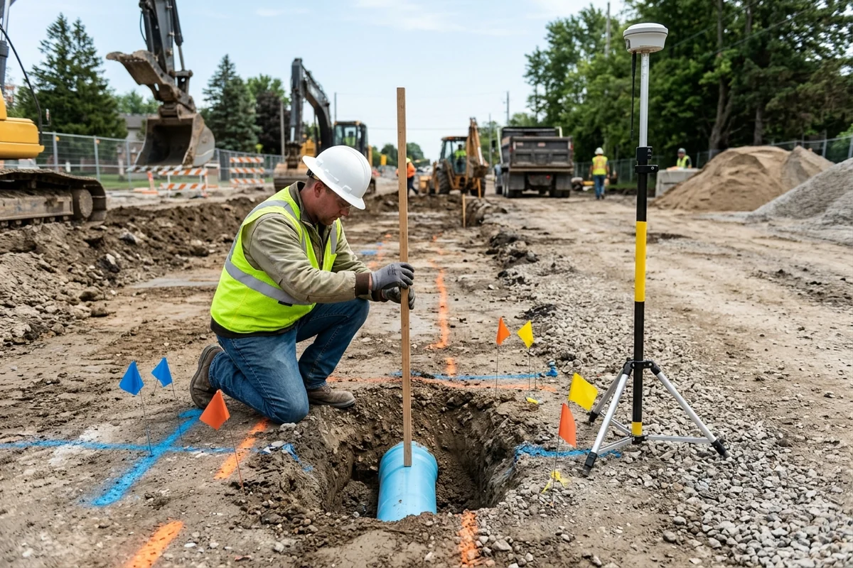
Temporary paint stripes and pin flags placed during One-Call 811 responses and SUE designating follow the American Public Works Association (APWA) uniform color code. As codified in state damage-prevention statutes such as the Colorado OPS Best Practice for Locating and Marking (referencing Common Ground Alliance Best Practices 18.0), pink markings cover temporary survey and engineer-placed SUE designations so geophysical investigation marks stay distinct from facility-owner 811 marks.
| APWA color | Marked utility or field activity |
|---|---|
| White | Proposed excavation limits |
| Pink | Temporary survey markings (including engineer-placed SUE marks) |
| Red | Electric power lines, cables, conduit, and lighting cables |
| Yellow | Gas, oil, steam, petroleum, or gaseous materials |
| Orange | Communication, alarm or signal lines, cables, or conduit |
| Blue | Potable water |
| Purple | Reclaimed water, irrigation, and slurry lines |
| Green | Sewers and drain lines |
Color-coded surface marks communicate horizontal corridor position only—never guaranteed burial depth. Nationwide, one in three underground utility strikes stems from digging without a prior 811 ticket; under Maryland’s Miss Utility rules, excavators must notify 811 at least two full business days—and no more than ten days—before breaking ground. Because frost heave, regrading, and erosion alter cover depth over time, crews must hand dig with shovels inside tolerance zones and keep mechanical buckets clear of painted alignments until lines are visually exposed.
Electronic depth readouts from EM receivers or uncalibrated GPR scans carry the same field caveat: Colorado’s locating best practices specify that electronic depth estimates are never guaranteed and must be confirmed through potholing, with the excavator notifying 811 immediately if a marked facility cannot be found in the test hole or sits outside its marked corridor.
What drives GPR survey scope and effort?
Utility mapping contracts rarely rely on a single flat site fee because field time scales directly with corridor congestion and verification tier. In the FHWA Purdue University SUE cost-savings study evaluating 71 highway projects exceeding $1 billion across Virginia, North Carolina, Texas, and Ohio, obtaining combined QL-B geophysical designating and QL-A test-hole data cost less than 0.5% of total construction value (about 1% to 2% of state DOT engineering and construction budgets) and returned $4.62 in quantified savings for every $1.00 spent—cutting overall construction costs by 1.9% compared with relying on QL-C and QL-D records alone. State DOT SUE programs commonly procure these investigations through unit-price schedules that separate surface geophysical designating (by crew day or corridor footage) from per-hole vacuum potholing, making scope adjustments auditable when field conditions shift:
- Grid density and bidirectional passes: Tightening a polarized x- and y-grid from standard 5 ft (1.5 m) spacing to 2 ft (0.6 m) high-resolution spacing more than doubles linear cart mileage across an intersection or utility trench corridor compared with 5 to 20 ft reconnaissance sweeps.
- Multi-frequency passes and manual radargram picking: Corridors stacking shallow telecom ducts above deeper water or sewer mains often require dual-frequency or multi-pass runs, followed by manual hyperbola picking rather than automated batch detection.
- Clay attenuation and internal nonmetallic tracing: Wet or clay-capped subgrades that block radar below 2 to 4 ft shift crew hours toward opening manholes and cleanouts to feed conductive fish tapes or push transmitting sondes marked every 5 to 20 ft.
- Velocity calibration and QL-A test-hole count: Pulling soil cores for permittivity calibration and vacuum-excavating conflict crossings (typically capped at 15 in. / 375 mm nominal hole diameter and surveyed to 15 mm vertical tolerance under DOT SUE scopes) add vacuum-truck mobilization, traffic control, pavement restoration, and survey crew hours per exposed crossing.
Field checklist for GPR grids, soil limits, and pothole exposure
Run through these six acceptance checks before signing off on pre-excavation utility sweeps or releasing mechanical trenching crews.
| Verification stage | Field acceptance check |
|---|---|
| 811 notice and record baseline | Confirm advance 811 ticket timing (at least two full business days and no more than ten days before digging under Maryland’s Miss Utility guidance) and treat unverified utility drawings or oral recollections strictly as Quality Level D. |
| Soil moisture and clay check | Evaluate clay cover and moisture ahead of mobilization; expect wet clay to mask lines deeper than 2 to 4 ft on utility GPR and conductivity above 30 to 40 mS/m to hold penetration well below 1 m. |
| Complementary EM and sonde sweep | Run active and passive EM locating on continuous metal and tracer-wired utilities, push a fish tape or sonde through accessible PVC, fiberglass, or vitrified clay pipes, and never treat a quiet passive 60 Hz scan as proof an electric cable is dead. |
| Polarized bidirectional GPR grid | Collect GPR passes in both x- and y-directions perpendicular to pipe trends at 5 ft (1.5 m) spacing—or 2 ft (0.6 m) in congested zones—and confirm pipe alignments across multiple crossings rather than marking a single B-scan hyperbola. |
| Metal shadow and concrete review | Flag steel pipes and road plates as total reflectors that blind GPR to deeper utilities underneath, and cross-check concrete storm or sewer alignments whose 4 to 11 permittivity blends into 4 to 30 native soils. |
| Pothole depth confirmation | Treat surface paint and flags as Quality Level B horizontal marks with no guaranteed depth; hand dig inside tolerance zones, vacuum-pothole conflict crossings to achieve 15 mm vertical Quality Level A survey confirmation at the test hole, and contact 811 if a marked line is missing. |
Sources
- FHWA InfoTechnology — Ground-Penetrating Radar (GPR) for Underground Utility and Concrete Investigation
- FHWA InfoTechnology — Ground-Penetrating Radar (GPR) for Bridge Decks
- FHWA — Avoiding Utility Relocations, Section IV: Subsurface Utility Locating Technologies
- USGS Circular 1310 — Surface Geophysics for Sand and Gravel Resources (Ground-Penetrating Radar)
- ASTM D6432-19 — Standard Guide for Using the Surface Ground Penetrating Radar Method for Subsurface Investigation
- NIST IR 89-3915 — Electromagnetic Techniques for Detecting Buried Objects
- Delaware DOT Engineering Instruction EI UT-20-001 — Displaying Utility Information Within the Plan Set (ASCE 38-22 Quality Levels)
- FHWA — Subsurface Utility Engineering (SUE) Program Overview and Quality Levels
- FHWA — Purdue University Study: Cost Savings on Highway Projects Utilizing Subsurface Utility Engineering
- FHWA Every Day Counts (EDC-8) — Subsurface Utility Engineering
- Maryland Office of People’s Counsel — Miss Utility 811 and APWA Color Code Guidance
- Colorado Office of Pipeline Safety — Best Practice for Locating and Marking Underground Facilities
Explore the related topic and technical references.